5 Direct Aerosol – Ammonia Interactions

5.1 Introduction

Ammonia is the primary base gas in the atmosphere, and as such is chemically very important. Because of its high solubility it is readily deposited to surfaces from the gas phase. This gives it an atmospheric lifetime of less than a day under certain circumstances. However, there are a series of reactions that can cause ammonia to enter the aerosol phase, leading to a variety of effects.

The ammonium ion (NH₄⁺; readily produced from NH₃) reacts readily with atmospheric gas phase acids to produce ammonium salts. These reactions occur rapidly on pre-existing aerosol, causing growth, or can stimulate aerosol production; these processes being collectively known as gas  particle inter-conversion processes. The commonest reactions are shown below. This is by no means a complete picture of ammonia – aerosol chemistry, but does show the reactions thought to be most relevant to this situation.

k_NH4Cl

NH_3(g) + HCl_(g) NH₄Cl_(s)

k_NH4NO3

NH_3(g) + HNO_3(g) NH₄NO_3(s)

k_NH4HSO4

NH_3(g) + H₂SO_4(g) NH₄HSO_4(s)

k_(NH4)2SO4

2(NH_3(g)) + H₂SO_4(g) (NH₄)₂SO_4(s)

k_s

i.e. Ammonia + Acid Ammonium Salt

It is worth noting that in the reactions shown involving Hydrochloric and Nitric acids, an equilibrium is set up, so that any surface aerosol mass produced by these salts would undergo volatilisation, were the aerosol to move into a region of lower acid or ammonia concentration. The sulphuric acid / ammonia – ammonium bi-sulphate reaction is also a reversible equilibrium. However, the final reaction, producing Ammonium Sulphate is not reversible. It is for this reason that appreciable amounts of Ammonium Sulphate are often found in ambient aerosol, and that this may therefore represent the most important of the above reactions for long-range transport of reduced nitrogen compounds. These reactions and their kinetics are investigated in more detail in a later section. The rate constants k_s are not given here since the determination of the rate of gas – particle inter-conversion is achieved using a time independent approximation (equations 5.1 – 5.4).

In the context of the GRAMINAE integrated experiment, the reactions listed above lead to ammonia flux divergence in the surface layer in conditions of ammonia emission. In order to confidently apply the gradient flux calculation method to ammonia emissions it is, therefore, necessary to make an assessment of the error induced in the flux calculation by this chemistry. This can only be done directly by measuring the rate of ammonia uptake to aerosol, which was to be inferred from the aerosol flux and concentration measurements described here.

The effects of ammonia emission on aerosol are especially important, as they can increase the atmospheric residence time of reduced nitrogen compounds from the order of several hours to several days when incorporated into fine / accumulation mode aerosol. This radically alters the transport properties of the compounds, in that long-range transport becomes possible. Aerosol effects are accordingly very important to certain aspects of the GRAMINAE project, as this process will contribute to trans-boundary air pollution, linking the climatic, chemical, microphysical and health effects of aerosol to the subject of ammonia emission.

Long-range transport of ammonia (facilitated by incorporation into aerosol) may be important due to its environmental effects. The presence of ammonia facilitates the incorporation of acid gases into aerosol, thereby similarly increasing their atmospheric residence times. Also, ammonia is implicated in the eutrophication (nutrient overloading) of sensitive ecosystems.

5.1.1 Measurements

The measurement site and instrumentation is described in the previous chapter on aerosol deposition and in Sutton et. al. (2002). The only additional required here is the treatment of the DMPS aerosol size distributions. The DMPS spectra are produced by combining two overlapping distributions from two differential mobility analysers (see Williams, 2000 for a full description of the DMPS). Although the two halves should be equal where they overlap, there were some periods during this experiment where this was not the case. This was thought, primarily, to be due to power distribution problems.

As part of the quality control of the DMPS data, the two halves of each size distribution were scaled so that they were equal in the overlapping region. The entire distribution was then integrated and rescaled so that the total aerosol concentration (D_p > 11 nm) reported by the DMPS was equal to the concentration measured by the CPC flux system. This procedure solved the intermittent mismatch between the two parts of the aerosol concentration distribution, and had the added advantage that in the following calculations, the data from the two systems was “coherent”.

5.2 Apparent emissions following fertiliser application

Figure 1 shows the time series of aerosol fluxes measured by the CPC system from the 5^th June (the day of fertilisation) to the end of the experiment. The ammonia fluxes measured using the gradient method are also included for comparison.

Both aerosol and ammonia emission are observed for around one week following fertiliser application, with the aerosol deposition returning on the 12^th June. Before that date, the diurnal cycle of aerosol and ammonia emission are co-incident. In interpreting the aerosol fluxes, the first question to be addressed is the nature of the process leading to the observed emissions.

5.2.1 Mechanism of aerosol growth

It is clear that the aerosol emissions are connected to the ammonia emissions. The systematic upward flux of aerosol was not observed until after fertilisation, when the large ammonia emissions began. There are, however, several mechanisms that could account for the observed upward aerosol fluxes. These are (Nemitz et. al., 2002 b)

1. Enhancement of the ternary production of (NH₄)₂SO₄ aerosol from the H₂O – H₂SO₄ – NH₃ system, with growth across the 11 nm cut off of the CPC system.

2. Formation of new NH₄NO₃ or NH₄Cl aerosol followed by growth across the 11 nm threshold.

3. Growth of existing aerosol by the combined surface condensation of NH₃ and HNO₃ or NH₃ and HCl.

Since production of (NH₄)₂SO₄ is enhanced at typical rural ammonia concentrations, and does not increase significantly with increases in ammonia concentration above the ng m^-3 range (Nemitz et. al., 2002 b), the first process is unlikely to be significant. The second and third processes would probably occur simultaneously, their relative importance being determined by the ambient aerosol population. In clean areas, new particle growth would be favoured, while in more polluted environments the species would condense onto the surface of any pre-existing aerosol.

5.3 Aerosol growth model

To test the likelihood of freshly nucleated particles ( 1  2 nm) growing to a detectable diameter (11 nm) in the layer of enhanced ammonia concentration above the experimental site, we can use the growth rate equation of Kulmala et. al. (2001) to estimate the time required for new particles to become detectable. A modified version of the equation is reproduced below.

(5.1)

Here m_v is the molecular mass of the condensing vapour, D is the diffusion coefficient, describing the Brownian diffusion of molecules onto the particle surface, _v is the concentration of condensable vapour species, r is particle radius, _p is the particle density and _m is a correction for vapour flux onto the particle surface for small aerosol. _m, the transitional regime mass flux correction factor, is estimated according to equation 5.2 (Fuchs and Sutugin, 1971). It is dependent on the Knudsen number (K_n; equation 5.3), the ratio of mean free path of the surrounding gas ( = 10^-7 m) to particle radius, and includes , an empirical sticking coefficient.  is thought to lie between 0.3 and 0.8 for NH₃ / HNO₃, (Dassios and Pandis, 1999; Cruz et. al., 2000; Rudolf et. al., 2001) and a value of 0.5 is used here.

(5.2)

(5.3)

Note that the diffusion coefficient used in equation 5.1 is not the same as that used in the particle deposition model. Here we are interested in the diffusion of gases onto the particle, rather than the diffusion of particles into surface roughness elements. Equation 5.4 shows the definition of the diffusion coefficient used in the particle growth model.

(5.4)

Results from equation 5.1 for an initial particle diameter of 1 nm are shown in figure 2. The growth rate of aerosol is not constant with time, as the condensable vapour mass flux to the particle surface is a function of D_p (from _m), and the growth rate at a given mass flux must also be a function of D_p. The figure gives an estimate of the time required for fresh aerosol to become detectable in the ammonia-enriched layer above the experimental site at various condensable vapour concentrations.

Figure 2 shows that it should take around six minutes for a freshly nucleated particle to grow to 11 nm, even at extremely high condensable vapour concentrations (_v = 20 g m^-3). With typical “fetches” of between 150 m and 500 m (chapter 4, figure 1) and a typical wind speed of 2 – 3 m s^-1, growth of freshly nucleated particles is very unlikely to be rapid enough to account for the observed emissions, even at very high vapour concentrations. In any case, the site was not remote from major regional aerosol sources (the conurbations and industrial activity typical of central Europe) and could not therefore be expected to be completely free of existing aerosol surface area to compete against nucleation for the available condensable vapour (chapter 4, figure 7 and table 4 show that average D₃ aerosol concentrations at the site were around 8000 cm^-3). Also, the DMPS measurements of size spectra (3 nm < D_p < 453 nm) showed no systematic increase in the nucleation mode (3 nm < D_p < 10 nm) concentrations following fertilisation. The third listed mechanism was therefore thought to be chiefly responsible for the measured aerosol fluxes.

That this growth mechanism was responsible for the aerosol fluxes means the interpretation of the flux as “emission” must be examined more closely. If large numbers of particles are not nucleated in the vapour rich layer above the fertilised field, there must be another explanation for the upward transport of particles larger than 11 nm. Figure 3 shows the postulated cause. That the gradient of particles smaller than 11 nm is constant with height is meant to indicate that approximately the same number of particles “grow into” this size range as grow to larger sizes from within this range, as explained below.

The total aerosol number concentration (and flux) across all sizes is unchanged by the condensable vapour emissions. The measured fluxes are a result of existing particles growing to a detectable diameter (11 nm in this case) in the lowest two metres of the surface layer,  below the measurement height. As the vapour concentration increases towards the surface, the gradient of detectable aerosol concentration becomes negative, resulting in an apparent emission of aerosol. So, there is no evidence of net production of aerosol, and the measured emission is indicative of growth rather than production. It is likely that very small numbers of particles may have been nucleated as a result of the vapour emissions, but as stated above, there was little evidence of this in the DMPS data, and it was hence unlikely to have been a major sink for the available vapour.

This being the case, the flux measurements can be used, in conjunction with the DMPS measurements, to estimate the growth rate of the aerosol, and hence the rate of transport of ammonia and nitrate into the aerosol phase and the associated error generated in the ammonia gradient measurements.

5.4 Availability of charge balancing ions

As determined above, the most likely mechanism for aerosol growth was the combined condensation of NH₃ and HNO₃ or NH₃ and HCl onto the surface of existing aerosol. The source of the ammonia to condense onto particles is clear;  figure 1 shows strong ammonia emission from the field following fertilisation. However, for aerosol to grow by the combined condensation mechanism, the number of ammonium ions removed to the aerosol phase must be matched by an equal number of nitrate or chloride ions, i.e. the charge balance of the particles must be maintained. Given the charges carried by the participating ions, the charge balance can be written as follows.

(5.5)

Where square brackets indicate the aerosol phase concentration of each of the major ions in each particle. The source of the negative ions to balance the ammonia uptake is less clear. These are all present in trace amounts in the atmosphere, but high concentrations would be required to account for the observed aerosol growth. An extension of figure 1 (below) suggests a possible source for the charge balancing ions.

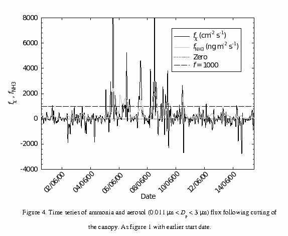
Figure 4 is similar to figure 1, except that the data begin on the 31^st June, the day the cut grass was lifted. Consistent ammonia emission was observed from this point onwards, with a clear diurnal cycle peaking during the day at the order of 300 ng m^-2 s^-1 (before fertilisation). The important point here is that similar systematic aerosol emission was not observed in the period between lifting of the grass and fertilisation of the site. The difference between ammonia emission from cut grass and ammonia emission from fertilisation may well have been the availability of the nitrate ion. Recall that the 100 kg N ha^-1 was distributed as pellets of calcium ammonium nitrate (CaNH₃NO₄). As suggested by the charge balance above (5.5), to maintain the ion balance of the pellets, ammonium and nitrate must evaporate or be washed out at approximately the same rate. Direct volatilisation of the fertiliser should therefore have not only drastically increased the ammonia concentration above the field, but also the nitrate concentration.

If, for the first week following fertilisation, a significant proportion of the ammonia emission was from direct volatilisation of the fertiliser, then there is an explanation for rapid aerosol growth not always accompanying ammonia emission (figure 4). The relationship between aerosol and ammonia fluxes and the (arbitrary) line at f = 1000 in figure 4 has an interesting property. When the diurnal maximum ammonia flux does not exceed 1000 ng m^-2 s^-1, we do not observe significant aerosol growth. The likely reason for this is that where the ammonia flux is below this level, it is being biogenically mediated. This predominantly means stomatal emissions, which would be of NH₄⁺ with no accompanying nitrate. Further evidence for this comes from the fact that where the ammonia flux is above 1000 ng m^-2 s^-1 there has generally also been weak nocturnal emission, which could only be a result of high surface / soil concentrations of ammonia,  i.e. fertiliser remaining on the leaf / soil surface.

So, it appears that significant aerosol growth is only detected in the presence of nitrate and ammonia emission. According to our current understanding, the bulk of the ammonia emission would initially have been direct volatilisation from the fertiliser pellets, until precipitation (on the 6^th and 7^th June) brought the fertiliser into solution on the plant leaves and in the soil. Nemitz et. al., 2002 (b) estimate that non-stomatal emission contributed to the ammonia flux up to five days after fertilisation, and this was also simulated using a “pasture simulation model” (PASSIM;  Riedo et. al., 2002). This estimate of 5 days coincides with the approximate end of large systematic aerosol “emission” on the 10^th June.

Unfortunately, the gradient measurements of HNO₃ were too uncertain for its fluxes to be calculated with any certainty for this project (Erisman et. al., 2002), however other work by Nemitz et. al. (2000) has showed positive gradients of HNO₃, and emission of HCl consistent with aerosol phase interaction of acids with ammonia. Further, van Oss et. al. (1998) attributed unexpectedly rapid deposition of nitrate aerosol to forest, to aerosol evaporation, while Nemitz et. al. (2002 c) made measurements of ammonium and aerosol flux over a Dutch heathland, obtaining results strongly suggestive of ammonium and nitrate participating in gas  particle inter-conversion processes. This at least establishes the plausibility of the proposed interaction mechanism.

5.5 Aerosol growth rate calculation

Having postulated simultaneous condensation of NH₃ and NO₃^– (presumably as HNO₃) as the likely aerosol growth mechanism, we need to calculate the growth rates to properly assess the effect of vapour emission on the aerosol population and ammonia gradient measurements. This is done using the flux conservation equation for the CPC system’s diameter range as presented by Nemitz et. al. (2002 b), but using D_p rather than particle radius for consistency

(5.6)

where  is aerosol concentration in the range 11 nm < D_p < 3 m, except that all terms enclosed in brackets refer to the diameter indicated in the subscript to the right of the term. For practical purposes, the far right hand term (at 3 m) can be neglected since the low concentration of super-micron particles makes it vanishingly small compared to the 11 nm term.

can be derived from the size distribution measurements of the DMPS. An estimate of the flux change with height is made using the average deposition velocity (v_d) to short canopy before the fertiliser was applied. Using the definition of deposition velocity and the interpretation thereof outlined in chapter 2, it is reasonable to assume that, approximately

(5.7)

Equations 4.11 and 4.12 can therefore be used in conjunction with measured data to estimate the growth rate across the lower cut-off diameter of the CPC flux system (11 nm). This allows solution of equation 5.1 for _v, to give an “effective vapour concentration”, – the concentration of vapour available for condensation given the ion balance limitation discussed above with respect to equation 5.5. Having determined the effective condensable vapour concentration, 5.1 can again be used to determine the aerosol growth rate as a function of D_p, with the total mass flux of vapour into the aerosol phase j_v then calculated according to the following (adapted from Nemitz et. al., 2002 b)

(5.8)

where r is particle radius (= ½ D_p) and all other quantities are as defined previously. The index “i” represents the particle size classes used in the calculation. In this calculation, j_v represents the mass flux of all vapour into the aerosol phase. Assuming that the growth is entirely due to NH₄NO₃ addition, the ammonia flux into the aerosol phase can be shown to be 21.28% of j_v (the molecular mass ratio of NH₃ to NH₄NO₃). This figure can then be related to the ammonia gradients, to assess the error that the combined condensation of these two species induces in the ammonia flux calculations (see Nemitz et. al., 2002 b for these error estimates).

Note that all of these calculations can be made without recourse to measurements of HNO₃ or NH₃ concentration or flux. A small number of simplifying assumptions have allowed the extent of aerosol phase chemical reactions to be estimated here solely from the aerosol measurements. The major assumptions are listed here, giving some idea of the validity of the scheme, and the limits of what can be deduced from the results.

1. Ammonia and nitrate are assumed to be the only species condensing onto the aerosol. Other ions such as chloride and sulphate are neglected.

2. The growth rate of aerosol across the 11 nm cut-off of the CPC system is used to calculate the effective vapour concentration, and this is used to calculate the growth rate at all other diameters.

3. In the flux conservation equation (5.6), the growth of aerosol across the 3 m upper cut-off of the CPC system is neglected as a sink of aerosol from the 11 nm < D_p < 3 m range.

4. is estimated (equation 5.7) from the difference between the measured aerosol flux and the deposition which would be observed if the average deposition velocity over short canopy was operating. The aerodynamic and surface resistances of the canopy are therefore assumed to be constant.

Assumption “1” can be justified from the point of view that the concentration of ammonia following fertilisation was very high compared to ambient gas phase chloride and sulphate concentrations (all of the ions mentioned had fairly stable concentrations throughout the whole project, while fertilisation gave rise to large ammonia concentrations and fluxes). In any case, calculation of nitrate loss is not the object of the scheme presented here. There may well have been a limited amount of condensation of non-nitrate ions onto the existing aerosol surface, but the effect of this would be taken into account by the use of “effective vapour concentration”.

There is reason to believe that assumption “2” is valid. The effective concentration represents the driving force for the condensation at 11 nm, and since the composition of the air was the same in the vicinity of all size fractions of aerosol, it should represent the potential for condensation at all sizes. It also has the advantage that the rate of condensation can be adequately approximated without detailed knowledge of every possible reaction taking place.

As stated above, the low concentration of super-micron aerosol means that, for example, even the loss of all aerosol in the size range 1 m < D_p < 3 m would have little effect on the total number concentration measured by the CPC system, hence assumption “3” is also reasonable. In any case, although the rate of condensation is expected to increase in proportion to particle surface area (D_p²), growth decreases proportionally to particle volume (D_p^-3) for a given vapour flux, giving an overall proportionality of diameter growth rate as D_p^-1. This means that large particles grow less rapidly than small ones, and the condensational loss rate of large particles from the range is hence expected to be lower than that of fine mode particles.

Finally, assumption “4” is expected to be valid since the aerodynamic and surface resistances of the canopy are expected to be governed by canopy morphology, which was virtually unchanged between cutting and fertilisation. Here the effect of canopy derived moisture is also noted. According to Kowalski (2001), deliquescence effects due to release or uptake of water vapour by the surface have an effect on fluxes measured by eddy covariance. However, there is no reason to suppose that this effect would be different before and after fertilisation, so the effect should be cancelled out by the use of equation 5.7.

5.6 Aerosol growth results

Figure 5 shows the calculated growth rates for 11nm and 200 nm particles, averaged over each day following fertilisation. Night time values are not shown in this figure, – they are treated separately later. The main feature to note in this figure is that the particle growth rates decline on average, settling to near zero growth at around 5 – 6 days after fertilisation (5^th June). The ratio of the diameter growth rates at 11 nm and 200 nm is fixed by equation 4.6 at a value of R_g = 22.7 where

(5.9)

The peak in growth rate on the 8^th June coincides with the highest diurnal peak in ammonia flux observed, except for the short period when the fertiliser was being applied on the 5^th June (figure 4). The 8^th June was the least cloudy and warmest day since before fertilisation according to the nearby DWD (Deutsche Wetter Dienst; –German Weather Service) measurements of global radiation, cloud fraction and air temperature. The large ammonia flux is attributed to the instability on the 8^th June, – it was also the least stable day of the whole project with average stability parameter  = 10 during the day.

The large calculated growth rate on the 8^th June is due to the large measured aerosol emission flux (average f_ during the day was 2077 cm^-2 s^-1, with emission velocity v_e = 3.43 mm s^-1). This is likely to be representative of rapid particle growth within the canopy, where the ammonia concentration was calculated to be around 75 g m^-3. This figure is extrapolated from the concentration at 1 m using the measured ammonia flux according to

(5.10)

where z₀’ is the zero plane displacement for ammonia concentration, or notional canopy height, the distance above the surface where zero concentration would be predicted during deposition, here acting as the effective source height. z_m is the measurement height (in this case 1 m for ammonia measurements), and r_a and r_b are the aerodynamic and surface boundary layer resistances as defined in chapter 2.

Negative particle growth rates are occasionally shown in figure 5; – this does not necessarily indicate evaporation of material out of the aerosol phase. It can be explained by one of two possible effects. First, the absence of significant particle growth along with v_d, the aerosol deposition velocity being higher than the average value during the short canopy period. This would cause the estimate of df_/dz (equation 5.7) to become negative, and is quite possible given that the first instance of this happening is on the 9^th June, 11 days after the canopy was cut. This gives ample time for the canopy to grow, increasing z₀ and leaf area index, which would tend to enhance aerosol deposition (see the previous chapter’s section on the Zhang et. al. (2001) deposition model). In fact, the canopy height had approximately doubled by the 6^th June, from 7 cm  3cm after the cut to 14 cm  3cm.

The second possible cause of negative estimates of growth rate is in the calculation of d/dr. If the gradient of the aerosol concentration distribution is negative in the region below 11 nm then this propagates into equation 5.6 (similarly to negative df/dz) making the growth rate calculation negative. This is the cause of the slightly negative growth rate shown in figure 5 on the 9^th June, and also of the low growth rate on the 7^th June.

Particle growth is only observed during the first five days following fertilisation. This is in line with the discussion above on growth mechanisms, and again, with the finding of Riedo et. al. (2002) that direct volatilisation of material from the fertiliser pellets lasts only five days.

Finally, with reference to figure 5, the rate of aerosol growth is rather high. Kulmala et. al. (2001) report growth rates for 1 – 3 nm particles of between 4 and 8 nm hr^-1 (radius growth of between 2 and 4 nm hr^-1) based on observations made above a boreal forest. The diameter growth rates estimated here range from near zero to, on average for the 8^th June, 3490 nm hr^-1 for 11 nm particles, and 154 nm hr^-1 for 200 nm particles (note that the diameter dependence of growth rate means that 1 – 3 nm particles would be expected to grow even more rapidly than 11 nm particles). These are higher than any “non-anthropogenic” growth rates reported in the literature, so particle growth following fertiliser application certainly appears to have an appreciable effect on the local aerosol population.

Given the growth rate equation (5.1) it is possible to simulate the effect of aerosol growth on the evolution of the aerosol population. Figure 6 shows the aerosol number distribution measured on the 2^nd June at 1800 GMT, and the same distribution “grown” for one cycle using a condensable vapour concentration of 2310 g m^-3, the value determined from the measured growth rate at 11 nm on 5^th June at 1300 GMT. The two distributions are similar except in the fine mode, where the effect of particle growth is clearly observable. Here, one growth “cycle” is, by definition, the amount of growth required to account for the observed upward aerosol transport. Recall that the growth rate is calculated from the measured flux according to equation 5.7; – the growth in one cycle is therefore identically equal to that inferred from the aerosol fluxes. An explanation for the use of the term “cycle” is reserved for a later section.

The third trace in figure 6 is the total mass flux of vapour into the aerosol phase as a function of particle diameter. Although the overall growth rate is proportional to D_p^-1, the vapour mass flux to a given particle is proportional to D_p². This causes the mass flux to peak at 85 nm for this distribution, – a balance between the increase with diameter of vapour mass flux per particle, and the decline in total aerosol surface area at larger diameters.

The calculations on which figure 6 is based are approximate. Since growth was only simulated for one cycle, the non-linearity of growth rate with time (figure 2) was neglected. For the calculations, the number distribution was converted to mass (rather than diameter) space, the mass flux, j_v, at each size was then calculated according to equation 5.1 and added to the distribution. Finally the modified spectrum was transformed back into diameter co-ordinates.

Figure 6 can be interpreted as the expected change to the aerosol distribution caused by the presence of fertiliser in the field. The un-modified distribution acts as the “upwind” aerosol population, as it was measured before fertilisation. The modified distribution is that which would have been measured following fertilisation given the same upwind distribution, after one “pass” through the canopy. Approximately then, the two distributions can be seen as “upwind” and “downwind”, giving an impression of the effect of fertilisation on the aerosol population at the downwind edge of the field.

5.7 Location of aerosol growth

Another question of interest is whether it can be determined where the aerosol growth is taking place. We know that the bulk of the condensation at all diameters must occur below the measurement height of 2.02 m in order to produce the observed upward fluxes, but an examination of the effective vapour concentrations gives a further insight. There is little value in using plots of _veff, as they follow exactly the same trend as the particle growth rates (figure 5). The values are presented in table 1, where negative values (deposition fluxes, see above) are presented but should probably be interpreted as “ 0 g m^-3”. As noted previously, the net contribution of deliquescence effects to the calculated growth rates should be insignificant.

Entries in table 1 are separated into day and night. Here “day” is defined as the period between 0400 and 1600 GMT (0600 to 1800 CEST, – local time), and “night” is defined as 1600 to 0400 GMT. This is the same definition used in figure 5, where only daytime values are displayed.

Table 1. Post-fertilisation day / night time averages of some major parameters associated with the aerosol growth rate calculations. All parameters as listed previously, except that j_NH4NO3 is the calculated mass flux of all vapour into the aerosol phase (assumed to be only NH₄NO₃, as explained previously). _veff is the calculated effective vapour concentration, _NH3 and _HNO3 are the measured acid and ammonia concentrations at z_m = 1 m and k_m/k_e is the ration of the measured concentration product to the theoretical dissociation constant for NH₄NO₃. “N/A” indicates that measurements are unavailable due to instrument malfunction.

The ratio presented in the final column in table 1 is important because it gives information on whether condensational growth should be possible. The quantities (k_m and k_e) are defined as

(5.11)

(5.12)

where T_a (5.12) is the absolute air temperature. Equation 5.12 is taken from Mozurkewich et. al. (1993), and represents the theoretical partial pressure product (in nb²) in equilibrium with the aerosol phase. k_e can only be calculated approximately here, as it is a function of aerosol composition, and information on internal vs. external mixing was not gathered (and no adequate method has been found for accurately predicting k_e for mixed composition particles). The values in table 1 are calculated for pure NH₄NO₃ particles, and as such, may be an over-estimate. Equation 5.11 represents the product of the partial pressures of ammonia and nitric acid, each again in nb. The partial pressure is calculated from the measured air concentration according to

(5.13)

where p[i] is the partial pressure of species i, N_i is the number of moles of species i present per unit volume, N_air is the number of moles of air per unit volume, and p is atmospheric pressure. In these calculations, atmospheric pressure is assumed to be constant at 1013.2 hPa, and air temperature is fixed at 20 C.

Aerosol growth is expected when the gas phase concentration product of ammonia and nitric acid (k_m) is higher than the equilibrium value (k_e). It is clear from table 1 that at 1 m, the height of the ammonia and nitric acid concentration measurements, aerosol growth is not expected (because in general k_m/k_e << 1). As noted above, given the large fluxes of ammonia observed following fertilisation, the concentration of ammonia within the canopy is significantly higher than that observed at 1 m (equation 5.10). The concentration products within the canopy are not calculated here, because in the absence of reliable acid flux measurements it is not possible to extrapolate the HNO₃ concentration at canopy height. However, it is clear that the concentration products must be significantly higher within the canopy than at z = 1 m.

This gives a reasonable indication of the location of the bulk of the aerosol growth. If aerosol growth is not expected at z  ½ z_m (= 1 m; z_m here relates to the aerosol measurement height) and it is clear from the ammonia flux measurements that the potential for particle growth must increase rapidly in the vicinity of the canopy (provided there was not significant deposition of HNO₃) it appears that the particles must have been growing inside the canopy, then being transported to the measurement height before having time to re-evaporate. This is the reason for the use of the word “cycle” in describing the duration of aerosol growth simulated in figure 6. The intention is to imply one cycle of a process where unmodified aerosol passes into the canopy, grows by condensation, and is then transported to z_m = 2.02 m. One cycle is specified, as it is envisaged that individual particles could make several passes through the canopy in the time taken for them to advect across the full extent of the fetch ( 500 m – 1000 m).

Although the analysis of turbulence time scales for the GRAMINAE field project (e.g. Nemitz et. al., 2002 d) is not yet complete, figure 7 shows early results, which support the hypothesis that aerosol can grow within the canopy and yet be transported to appreciable heights without re-evaporating. All the parameters shown indicate, in some way, the intensity of turbulence within the canopy and slightly above it. In every case, the measurements suggest that the intensity of turbulence is reduced within the canopy, and therefore that the timescale for pollutant transport is increased. This may mean that although the timescales for aerosol growth and evaporation are expected to be approximately comparable, the canopy is able to have a net effect on the aerosol population as measured at z = 2.02 m. Note that these measurements were made inside the long canopy, however the results are expected to scale down to the lower canopy height following cutting and fertilisation.

The results shown in figure 7 are verified by measurements of Radon diffusivity (Lehmann et. al., 2002), which were observed to decrease towards the bottom of the canopy. The Radon “tracer” results also indicated a similar effect in the short canopy, giving some confidence that the anemometry results should also scale down to the short canopy.

5.8 Summary of results

Fertilisation of the experimental grassland was shown to cause aerosol growth, the postulated cause being simultaneous condensation of ammonia and nitric acid onto the surface of existing particles. Diameter growth rates at 11 nm were calculated to range between zero and around 3490 nm hr^-1, with growth rates at 200 nm fixed at 22.7 times lower than those at 11 nm.

Evidence has been presented suggesting that the presence of the canopy may be an important factor in the growth of aerosol, with the time scale of turbulence being large within the canopy (low eddy diffusivity), allowing time for growth before rapid mixing to the measurement height.