6 Urban Aerosol Fluxes
6.1 Introduction
Urban aerosol is a topic of current interest (e.g. Colvile et. al. 2001, Harrison and Yin 2000, Fenger 1999, Mayer 1999, Micallef and Colls 1998) because of the climate forcing caused by aerosol, and because of rapidly increasing global urban populations. It is thought that around half of the word’s population currently live in cities, with global population still rising rapidly, especially in the developing world (Fenger, 1999).
Much attention has recently been given to urban aerosol and its likely injurious effect upon human health. Schwarz (1994) showed that for a 100 g m-3 increase in total suspended particulate mass (TSP) concentration, the relative daily risk of mortality was increased by 6% in a meta-analysis of data from studies in North America and Europe. It is noted that, with respect to the epidemiology carried out after the London “smog” of December 1952, while the mechanism of interaction between particulate material and human health is not understood, there is very little doubt that the interaction takes place.
In studies based on PM10 concentrations it has been estimated that around 6% of all urban mortality is attributable to air pollution (Künzli et. al., 2000). Furthermore, mortality is more closely associated with PM10 than with other candidates such as TSP, NO2, SO2 or aerosol acidity (Dockery et. al., 1993). PM10 is defined as the total aerosol mass concentration associated with particles smaller than 10 m diameter, often also referred to as the “respirable fraction”.
The population groups principally at risk from aerosol pollution are the elderly and those with pre-existing cardio-pulmonary illness. This suggests that excess deaths reported in epidemiological studies are brought forward by, rather than wholly induced by pollution, and it is therefore difficult to assess the effect on individual lifespans (COMEAP, 2001).
The size fraction of aerosol responsible for health effects is difficult to establish from epidemiology alone, as all likely size fractions are often well correlated with each other, and because size distributions are generally not monitored. However, there is increasing speculation from toxicological research that fine aerosol are particularly harmful (e.g. Seaton et. al. 1995), which is understandable given the efficiency of aerosol in the range 10 nm < Dp < 100 nm at depositing in the deeper regions of the lung. Donaldson et. al. (1998) even suggest that otherwise benign substances can become pathogenic when deposited to the lung as particles smaller than around 50 nm, and go on to explore possible physiological mechanisms for the toxicity. Future European legislation is expected to be aimed at smaller size fractions, possibly down to PM0.1 or even to use particle number (Colville et. al., 2001). Measurements in the size range presented in this chapter are therefore relevant to the human health debate.
Cities act as sources of aerosol, and are likely to be important on a regional scale. Despite this, no direct measurements have been made of the rate of aerosol production and transport above cities. Many of the recent investigations have been devoted to measurements of PM10 and PM2.5 concentrations within cities, but making inferences from these measurements about the amount and character of aerosol leaving cities may be a source of error in assessments of the effect of cities on a regional scale.
The effects of urban aerosol outside their city of origin are many and varied. Aerosol deposit to land downwind of cities, on agricultural land and potentially sensitive ecosystems, modify the chemical and radiative (e.g. Jacovides et. al., 1997) properties of the downwind atmosphere and alter the regional cloud population (e.g. Hitzenberger et. al., 1999), depending upon their number, composition and size distribution. In order to make a proper assessment of the effect of the urban plume on atmospheric chemistry and microphysics, information is, at least, required on the number and size distribution of the aerosol rather than the more commonly measured mass loading.
Urban areas are made up of a variety of surface types and point sources of pollutants arranged in a very inhomogeneous manner. Typically, surfaces such as roads, buildings, parks and construction sites are found together in various densities in cities over the scale of eddy covariance measurements (of the order of a kilometre; figures 1 and 2). In the absence of direct flux measurements, determination of the spatial variability of sources within a city and the net emission due to those sources is an uncertain exercise, although interesting source apportionment analyses have been published on the basis of mass concentration measurements (e.g. Harrison et. al., 1997).
6.1.1 Measurement and Interpretation
This chapter presents measurements of aerosol number fluxes and concentrations made above the City of Edinburgh, Scotland’s capital and second largest city with a population of 450,000 inhabitants and covering an area of 261 km2. These results concern aerosol in the diameter range 11 nm < Dp < 3 m (later referred to as the D3 range), and are primarily representative of aerosol smaller than 100 nm. Much of the content of this chapter has been published (Dorsey et. al., 2002).
These direct measurements of aerosol fluxes above a city using the eddy correlation technique have been made with a view to providing more direct and reliable parameterisations of the effect of cities on the regional aerosol population and on the health of the inhabitants of cities. This chapter presents results from three periods of measurement in the centre of the City of Edinburgh (UK) and is concerned with the production and transport of aerosol in the D3 size range. The results of flux measurements are presented, and estimates made of urban emission velocities (the concept of emission velocity is also discussed in chapter two).
![]() (6.1)
(6.1)
![]() and
and
![]() (later denoted by
for simplicity) are the flux and concentration of species n,
calculated over an averaging period of 15 minutes (in this case),
respectively. Note that the definition of emission velocity is simply
the same as the commonly used deposition velocity with a sign
reversal. This was felt to be more appropriate for the current study
on aerosol production and emission as it differentiates from the
slightly different role of deposition velocity.
(later denoted by
for simplicity) are the flux and concentration of species n,
calculated over an averaging period of 15 minutes (in this case),
respectively. Note that the definition of emission velocity is simply
the same as the commonly used deposition velocity with a sign
reversal. This was felt to be more appropriate for the current study
on aerosol production and emission as it differentiates from the
slightly different role of deposition velocity.
The use of emission velocity in this chapter is not analogous to deposition velocity in the more familiar deposition studies (e.g. chapter four). In the latter case the deposition velocity is well characterised and is solely dependent upon the state of boundary layer turbulence. It has a fundamental physical meaning and can be used to calculate deposition fluxes accurately. The emission velocity used here does not determine the aerosol flux, which is a result of the rate of production. In this study, the emission velocity is used as an empirical measure of the vertical ventilation of particles from the city, and in the parameterisations to be described is used to ascribe the apparent influence of a non-anthropogenic source. As a measure of vertical ventilation rate, the use of emission velocity is entirely justified, but it must be remembered that the similarity between it and deposition velocity is superficial.
A large measurement height of 69 m was chosen, because here the individual small scale processes at the surface are expected to have been blended into a relatively homogeneous net plume. However, over a time-scale of 15 minutes in areas as inhomogeneous as cities there are bound to be some periods of instationarity in the data caused by advection. This is part of the nature of urban aerosol concentration and is unavoidable. In order to reduce the likelihood of significant errors being introduced into the flux measurements by these instationarities, both spectral and co-spectral analyses have been performed on the aerosol data. Periods have been excluded from the subsequent analysis where the spectral behaviour deviated significantly from the average.
6.1.2 Scope of the Analysis
The dependences of flux and emission velocity upon aerosol production (anthropogenic activity) and urban micrometeorology have been examined. The differences in aerosol production and transport between late spring and late autumn are discussed, and it is shown that the study city produces more aerosol during the autumn measurement campaigns than during spring.
The different surface types are shown to have a marked effect on measured aerosol emission fluxes, with parkland being a weaker aerosol source than other areas. The diurnal behaviour of fluxes and emission velocities are examined and related to seasonal changes and anthropogenic activity. In this study, the sole measure of anthropogenic activity used is the rate of traffic flow on the streets, since road traffic is the major source of urban aerosol by mass (EPAQS, 1995). The frequencies of different magnitudes of aerosol fluxes are shown, and related to meteorological conditions.
The relationship between D3 aerosol number flux and traffic activity is examined and quantified for the study city. This is followed by an examination of the effect of boundary layer stability on emission velocity. These relationships are combined to give a predictive parameterisation for urban D3 aerosol concentration
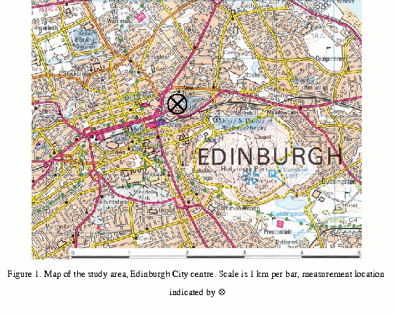
The city of Edinburgh was chosen as the measurement location. Measurements were made from an existing tower in the centre of the city. The Nelson Monument is a narrow circular stone tower, diameter approximately 4.5 m, standing 32 m tall. Its base is situated approximately 35 m above street level, giving an effective measurement height of 69 m (including the 2 m mast on which instruments were mounted). The mean building height in the West-South-Westerly city centre sector is approximately 15 m. The monument stands at the east end of the city centre, (310’52’’W 5557’17’’N, OSGB NT 26258 74134) and is surrounded by several surface types. The main areas are heavy urban, residential and parkland. This provided a good contrast between the emission properties of these different types of land cover during different wind directions.
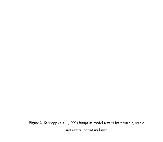
The location chosen has an urban or parkland fetch of at least 2 km in all directions, and in the prevailing westerly wind, the built up area extends some 7 km upwind. Figure 1 shows a map of the area, which will be used to inform interpretation of the results. A simple footprint model (Schuepp et. al. 1990) run using typical measured urban
micrometeorology shows,
in conjunction with figure 1, that for most atmospheric conditions
encountered in the study city the footprint covers mainly urban
surfaces. Results of this analysis are presented in figure 2 with the
following parameters used (typical urban values): friction velocity
u* = 0.4 m s-1, measurement height zm
= 70 m, zero plane displacement d = 10 m, roughness length z0
= 0.4 m and stability parameter, indicated in figure 2, in the range
–0.1 <
![]() < 2.0 where:
< 2.0 where:
![]() (6.2)
(6.2)
This relationship is also presented in chapter two, where zm = Measurement height (m), L = Obukhov length (m), d = Zero plane displacement (m).
Three measurement campaigns were conducted as part of the URGENT thematic programme (Urban Regeneration and the Environment) of the UK Natural Environment Research Council (NERC), this project being entitled Sources And Sinks of Urban Aerosol (SASUA). The first measurement campaign (SASUA I) took place from 12th – 27th May 1999 i.e. in late spring / early summer. The second and third campaigns (SASUA II and III) were run over 14th – 28th October 1999 and 26th October – 15th November 2000 respectively i.e. in autumn.
The aerosol flux data presented here were obtained using eddy covariance systems, mounted on top of the Nelson Monument at a measurement height of 69 m above street level. This chapter focuses exclusively on measurements and results from the UMIST CPC flux system, although various other measurements were made (these are published elsewhere). The CPC flux system is described in chapter three.

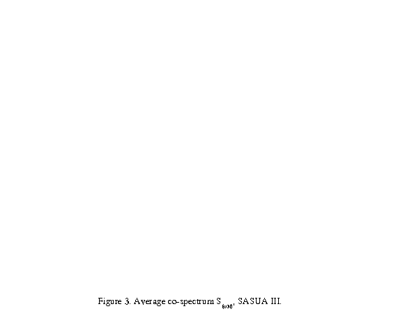
Laboratory tests have shown the CPC flux system to have a response time to large step changes in aerosol concentration of the order of 0.5 seconds. The analysis in chapter four confirms this, suggesting an upper frequency response limit of the order of 1 Hz, possibly up to better than 2 Hz under certain circumstances. Co-spectral analysis showed that the highest frequency eddies contributing to the flux at the measurement height had a period of significantly more than one second (figure 3), indicating that little or no loss in the measured flux would be expected with this system due to the instrument response time. Co-spectral analysis of accumulation mode aerosol fluxes measured at the same site, at the same time using an ASASP-X (DMT, Boulder, Colorado, USA) based aerosol flux measurement system (CEH, Edinburgh, UK) confirm the finding that the aerosol transporting eddies have a frequency greater than one second.
The information produced by the CPC flux system is limited to total aerosol number flux in the D3 size range. However, in an urban environment, concentrations and fluxes (hence emission velocities) in this size range are dominated by aerosol below 100 nm (in the urban environment) to such an extent that this instrument (and the urban D3 size range) is considered to have a practical upper cut off of 100 nm.
Figure 4 shows an example aerosol size spectrum taken during SASUA III using the Differential Mobility Particle Sizer (DMPS; described by Williams, 2000). It is an average of all readings taken over a period of six hours from 1200 – 1800 GMT on the 2nd November 2000. The distribution shown is typical of urban aerosol size spectra, and demonstrates the dominance of sub-100 nm aerosol of the total number concentration. Integration of the distribution below Dp = 100 nm yields a higher concentration by a factor of over 19 than above 100 nm in this case (i.e. the number concentration above 100 nm is 5.2% of that below 100 nm). Thus these number weighted measurements, referred to as the D3 size range are representative of the size range 11 nm < Dp < 100 nm.
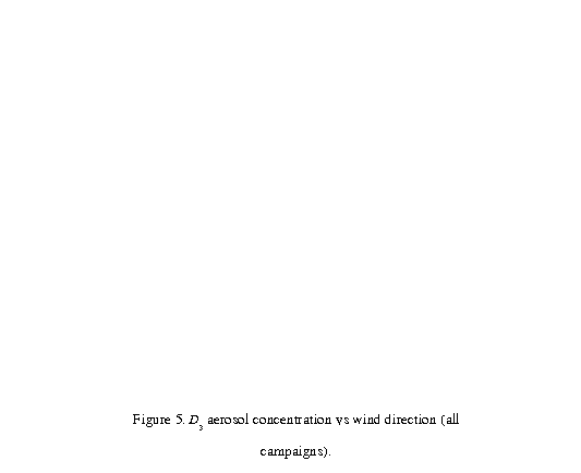
One of the major questions of interest during this project was the spatial variability of aerosol concentrations and fluxes as determined by the distribution of sources. Figure 5 shows the D3 aerosol concentration as a function of wind direction, all data averaged over all three campaigns.
The high concentrations measured in westerly winds are expected, as the city centre area lies in that direction (figure 1). In all directions, there is an observable relationship between high mean aerosol concentration and areas of heavy urbanisation and little parkland. Conversely, all wind directions giving comparatively low mean concentrations coincide with local parkland.
The aerosol fluxes, shown in figure 6 show a broadly similar distribution, although emission appears to be slightly depressed during easterly winds. This is attributed to lower local emissions in that direction and implies that in Easterly winds the site is affected more by background concentrations and less by local production than in Westerly winds. The average emission velocity measured in easterly winds was less than half that measured in westerly winds (of the order of 25 mm s-1, as opposed to 60 mm s-1, figure 6).
Apart from there being stronger local emission to the west of the measurement point, the rougher surface of the city centre is expected to enhance mechanical turbulent mixing. The surface drag coefficient can be defined by:
![]() (6.3)
(6.3)
and varies typically between 1 x 10⁻³ and 2 x 10⁻². Stull (1988) cites 1 x 10⁻³ to 5 x 10⁻³ as typical values for non-urban areas. The measured urban values are therefore very high compared to natural surfaces.
Figure 6 also shows the large variability in urban aerosol number fluxes. Values can be as high as 150,000 cm-2 s-1, although on rare occasions weak deposition is observed at night. Figure 7 is a histogram of number flux for all campaigns (744 hours of data).

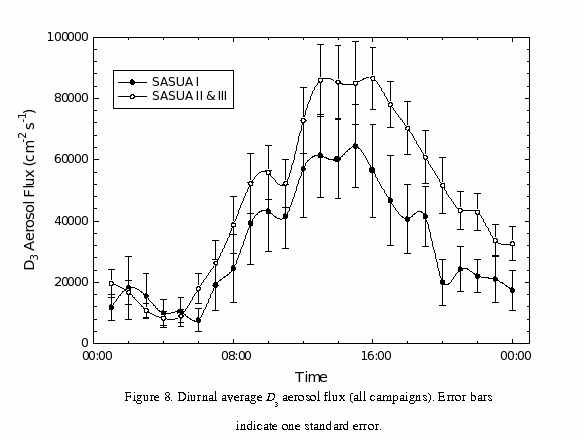
The distribution shown in figure 7 demonstrates that the city rarely acts as a net sink for small aerosol. Less than 6% of observed hours showed net deposition, and all deposition events were comparatively weak (low net fluxes). Apart from the dependence of D3 flux upon wind direction, there is a strong diurnal variation in concentration, flux and emission velocity. Figure 8 shows the aerosol flux, diurnally averaged over both SASUA I and SASUA II and III. The timebase in figure 8 is local time, so that the SASUA I data, in BST, is one hour ahead of solar time. This shift shows that since many features occur at the same time in the plots, anthropogenic activity dominates aerosol production. Examples include the morning rush hour and peak around noon, which occur at different times with respect to solar time, but at the same time according to local time.
The
aerosol flux is dependent on both aerosol production rate, – in
this case dominated by anthropogenic activity, and the
micrometeorological processes transporting aerosol. The fluxes
measured in the October campaigns are higher than those measured in
May. This is caused by an increased production rate. Road traffic
activity was significantly higher during the October 2000 campaign
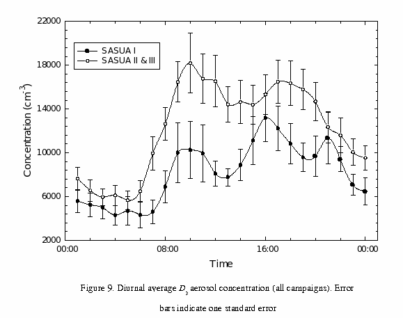
than SASUA I and II ( on average by 23.5%). Figure 9 shows the
diurnally averaged aerosol concentration from all campaigns. It shows
lower concentrations during the spring campaign, in agreement with
the lower production rate discussed above.

Figure 10 shows the dependence of aerosol fluxes on one important anthropogenic activity, – traffic movements in the city. Although road traffic is not the only source of aerosol within the city, and the production rate does not appear to solely determine the flux, a fairly good correlation can be seen between the rate of traffic movements and the aerosol emission. The intercept of the fit to the data with the zero traffic line indicates a background flux of around 12,000 cm-2 s-1 not attributable to road vehicles. This figure is between 15 – 20% of the peak fluxes indicated in the diurnal averages (figure 8), confirming that traffic activity is the dominant source of aerosol in the D3 range during the day.
The sources of this background flux are difficult to establish as the periods of low traffic activity are found exclusively at night. Possible nocturnal aerosol sources include combustion for space heating and non-road transport (rail). Photochemical secondary aerosol production mechanisms cannot operate at night, and there is no obvious source for large amounts of precursor gases in any case in the absence of traffic. It is therefore likely that the background flux consists of primary aerosol emitted by either of the other sources mentioned.
The traffic activity used here was recorded on one street within the city centre, but a very good linear correlation between all three traffic census points in the city has been found, so that for a qualitative analysis any measurement point could be used. This illustrates the difficulty of “scaling” urban observations. Vehicle usage is expected to differ between cities, and even in one city the traffic measurement location solely determines the range of observations, in that busy roads are an order of magnitude busier at all times than minor and residential roads.
During SASUA I and II the diurnal variation in traffic activity (provided by Edinburgh City Council) was typically between 200 and 2800 vehicles per hour on the stretch of road used. SASUA III has been excluded from this analysis due to the vastly different traffic activity observed. It would be difficult to put forward objective arguments for the use of one traffic census point rather than another anywhere in the city. For this study the nearest census point to the measurement location was used.
The fit to the data shown in figure 10 can be reproduced by the following parameterisation, where f = Aerosol flux (cm-2 s-1) and T = Traffic activity (vehicles per second at the Queen Street traffic census point, an arbitrarily chosen reference site):
![]() (6.4)
(6.4)
where the constants A = 13,000 and b = 1.6.
The diurnal variation in emission velocity over the city is of interest as it shows the range of typical values, and the effect of surface heating. Figure 11 shows the diurnally averaged D3 emission velocities for SASUA II and III.
Data from the May campaign (SASUA I) have not been presented in figure 11, as the lower number of samples collected resulted in a statistically less reliable average (mean standard deviation was 83% of the mean hourly value). The effect of heating is pronounced, with the emission velocity increasing from 20 mm s-1 at night to around 68 mm s-1 at solar noon. Note that this must be a result of increased transport, as a stronger aerosol concentration gradient caused by more rapid aerosol production would affect the flux but not the measured emission velocity to this extent.
There
was no strong dependence of mean wind speed on time of day. Edinburgh
is typically windy, with an average wind speed during SASUA III (the
“windiest” project) of 6.5 m s-1, so the
emission velocity of 20 mm s-1 at night is assumed to be
representative of the contribution to mixing of mechanically
generated turbulence, in the absence of surface heating. Emission
velocities measured in May tended to be higher (although fluxes were
generally lower), peaking at 75 mms-1 due to higher
surface heating and lower mean concentrations.
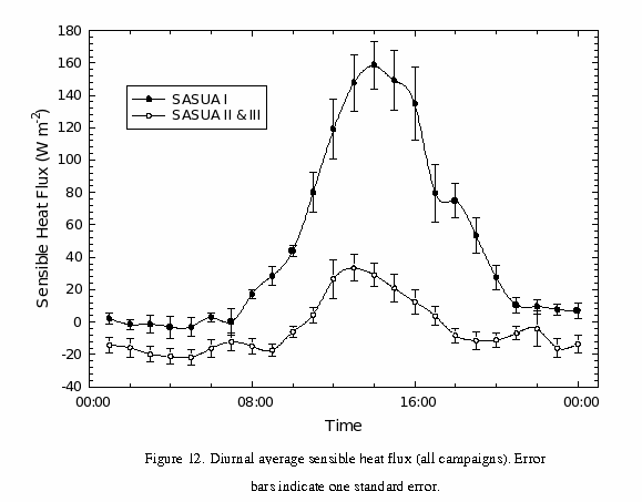
The seasonal difference in surface heating and hence buoyant vertical mixing is shown in figure 12. The sensible heat fluxes diurnally averaged over SASUA I and SASUA II and III are shown. The peak for the October campaigns is significantly lower than for May, and night time values are significantly below zero. The May average values do not often fall below zero, suggesting that the city is capable of storing heat on warm days, and releasing it throughout almost the whole night.
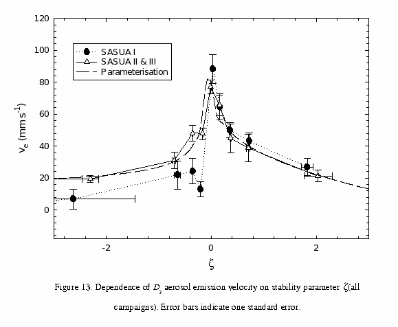
The
final dependence of aerosol emission velocity to be investigated here
is connected to sensible heat transport; – this is the
variability with atmospheric stability. Figure 13 shows the average
emission velocity for a range of the stability parameter .
Results are campaign averages and are presented separately for the
October and May campaigns. Note that positive values of
represent unstable conditions. It is expected that as
increases, the intensity of convection and hence vertical mixing will
increase.
![]()
![]() (6.5)
(6.5)
![]()
![]() (6.6)
(6.6)
The
parameterisation is based upon the average values for all three
campaigns, and follows the SASUA II and III behaviour most closely
because there were significantly more data available from these
periods. Since the equations are written in terms of emission
velocity rather than aerosol flux, the parameterisation should be
applicable to a first approximation for other cities of a similar
density and vertical scale.
Figure 13 also goes some way toward explaining the generally higher emission velocities observed during the May campaign. Due to increased insolation of the surface in May, sensible heat fluxes are higher and the boundary layer is, on average, less stable. This skews the stability parameter frequency distribution to less stable values (although it maintains a broadly similar shape). This effect is shown in figure 14.
 6.3.4 Bi-directionality
of Aerosol Fluxes
6.3.4 Bi-directionality
of Aerosol Fluxes
The shapes of the traces in figure 13 seem at first somewhat unexpected. The increase in emission velocity with increasing stability parameter up to around -0.25 is as expected due to decreased thermal suppression of vertical mixing. As the boundary layer becomes less stable, mixing is suppressed less and the emission velocity increases. The behaviour around the neutral limit of the stable regimen is not thought to be significant, with the bin widths chosen as much as anything else affecting the shape, – there is significant scatter in the data in this region.
There is evidence (Barlow and Belcher, 2001) that increased wind speeds can give rise to increased ventilation of urban canyon systems. Indeed, during this experiment it was noted that, in neutral conditions, emission velocity increased with wind speed on average. Since high wind speeds tend to coincide with neutral conditions it is possible that there is an element of this effect contributing to the shape observed in Figure 13. However, it is not thought that the effect is significant in this case. Directional analysis of the aerosol fluxes show that downward transport is increased during unstable conditions (see below), and suppression of transport out of canyons at low wind speeds would have to lead to unrealistically high street level concentrations to explain the observed pattern. In any case, the work of Barlow and Belcher (2001) was aimed at street canyon ventilation rather than city scale fluxes as investigated here.
In
the unstable regimen, emission velocity decreases with increasing
instability. This is thought to be a result of downward mixing from a
region above the measurement level. Aerosol from the top of the
boundary layer may be mixing downwards to the measurement height
during periods of very strong convection, and suppressing the
observed upward flux.
Negative
fluxes are not observed (in this type of ensemble average), as the
city is still acting as an aerosol source, however there is thought
to be a bi-directional flux causing weaker net emission to be
observed. Further experimental work is required to determine if this
is indeed the case, although figure 15 shows the postulated cause,
with a large build up of fine aerosol at the top of a polluted
boundary layer around noon. These data were derived from aircraft
measurements over the city of Birmingham during another NERC URGENT
project, Pollution of the Urban Midlands Atmosphere (PUMA).
Figure 15 shows the required upper layer of high aerosol concentration to explain suppression of the observed flux by a component of downward transport. The source of the aerosol is not well established, but it is thought that large numbers of aerosol are produced in inter-cloud regions at the top of the boundary layer (Keil and Wendisch, 2001). This could possibly explain certain ultra-fine particle bursts observed by Shi et. al. (2001) given the correlation they note between a particle burst and an increase in solar radiation. There is also a coincidental increase in wind speed in their data, possibly indicating a downburst of particle-laden air from the vicinity of a cloud that has passed, allowing solar radiation to increase.
From the point of view of the data from the SASUA campaigns, there is no unambiguous indication of the reason for the apparently bi-directional D3 aerosol fluxes. Figures 16 and 17 show a directional analysis of the variation in flux and emission velocity with boundary layer stability parameter. These fluxes and emission velocities were calculated using exactly the same method outlined in chapter two, except that the positive and negative portions of the instantaneous (w’’) covariance over each averaging period were separated and summed. They were then weighted with the frequency of positive and negative instantaneous covariances respectively, giving an estimate of the net, upward and downward fluxes of D3 aerosol.
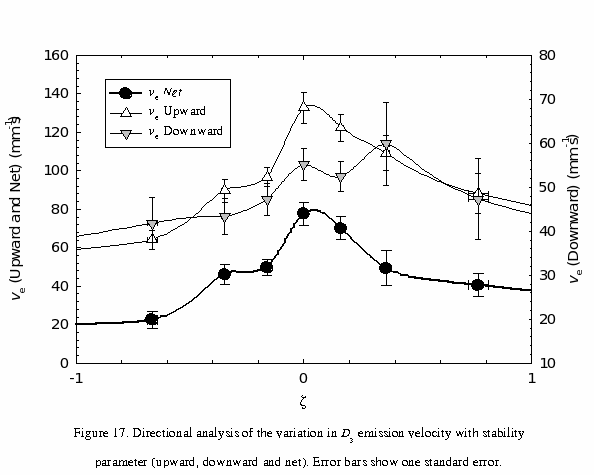
Although the relationship between concentration and the bi-directionality of flux and emission velocity is likely to be extremely complicated, there are identifiable features in figures 16 and 17. Significantly, the peak in downward aerosol flux (figure 16) appears at the same stability as the beginning of the downturn in net flux and the peak in upward flux. It is difficult to understand how this might happen in the absence of a source of aerosol aloft (again, as shown in figure 15).
Figure 17 shows that the peak in downward aerosol emission velocity (effectively a deposition velocity) peaks at a higher value of than the upward or net emission velocities. Interpretation of emission velocity is by no means straightforward in the presence of an aerosol source, let alone the hypothesised pair of opposing sources of differing strength. However, it is clear that figures 16 and 17 do not show the expected result of vertical mixing from a single source at the surface.
6.4 Aerosol Concentration Parameterisation
Given the parameterisations 6.4, 6.5 and 6.6 it is possible to approximate the urban D3 aerosol concentration () in the size range considered. Combining 6.4 with 6.5 and 6.6 and introducing an empirical wind speed dependence to allow for the effects of dilution in the vicinity of sources produces equations 6.7 and 6.8:
![]()
![]() (6.7)
(6.7)
![]()
![]() (6.8)
(6.8)
With
![]() = Mean wind Speed (m s-1) at the measurement height, all
other quantities as before (recall A = 13,000 and b =
1.6). Given the scatter visible in figures 10 and 13 showing the data
on which this parameterisation is based, equations 6.7 and 6.8 are
clearly only approximate. They are formulated solely in terms of
traffic activity and boundary layer stability, so there are clearly
processes missing. The main quantity omitted from the
parameterisation is the background concentration of aerosol advected
into the city.
= Mean wind Speed (m s-1) at the measurement height, all
other quantities as before (recall A = 13,000 and b =
1.6). Given the scatter visible in figures 10 and 13 showing the data
on which this parameterisation is based, equations 6.7 and 6.8 are
clearly only approximate. They are formulated solely in terms of
traffic activity and boundary layer stability, so there are clearly
processes missing. The main quantity omitted from the
parameterisation is the background concentration of aerosol advected
into the city.
In
its current form the parameterisation reproduces large portions of
the data reasonably well (figure 18), but suffers from spikes due to
coincident large values of traffic activity and stability parameter.
Over the course of all three city centre measurement campaigns the
parameterisation predicts 18% more particles than were observed. This
figure includes the effect of the spikes mentioned above. Figure 18
compares a portion of measured concentration data with the results of
the parameterisation for a period where it was fairly effective.
Although the results are by no means perfect, the parameterisation
can clearly reproduce certain aspects of the diurnal behaviour of
aerosol concentration.
The agreement shown in figure 18 means that two of the major processes determining urban aerosol concentration have been identified. The calculation is based solely on traffic activity, wind speed and boundary layer stability. Effectively the parameterisation describes production of aerosol and ventilation of the city. The concentration appears to be determined by the balance of these two processes. Note that as mentioned before, the traffic activity is essentially an arbitrary measure. In order to extend this parameterisation to other cities it would be necessary to find some more independent quantity by which to parameterise anthropogenic activity, or to introduce an empirical scaling factor on the traffic activity. This could be simply achieved by varying the factors A and b of equation 6.4, where for a denser street layout the factor b would probably need to be increased, and for a vehicle fleet producing more aerosol, A would be increased.
It is less clear how the constants originating in equations 6.5 and 6.6 would vary for different cities, and they have therefore been left as numerical values. It is likely that the constants from both equations would, for a given city, be some function of the local pollution climatology, distribution of fixed local sources and roughness length. Further work is required in a variety of cities to find the determinants of these constants as well as of A and b from equations 6.4, 6.7 and 6.8.
It is worth noting, with respect to this parameterisation, that traffic activity may act as a surrogate for other anthropogenic aerosol producing activities. However, a measurement based extension of the equations to other cities should be tenable, as any activity uncorrelated with traffic flow would be reflected in the constants originating from equations 6.5 and 6.6.
Measured values of aerosol concentration, number flux and emission velocity for a city have been presented for the D3 aerosol diameter range, where the measurements are known to be representative of the sub-100 nm size interval. The influence of land use type on these quantities has been discussed. It was found that heavy urbanisation is associated with higher aerosol emission velocities, fluxes and concentrations. Aerosol (D3) concentrations were found typically to range between 3,000 cm-3 and 20,000 cm-3 although larger values were observed. The mean D3 aerosol flux over the three campaigns was found to be 42,500 cm-2 s-1, with the mode being 30,000 cm-2 s-1 and the typically observed range was 9,000 cm-2 s-1 to 90,000 cm-2 s-1. The mean and mode emission velocities were 45 mm s-1 and 35 mm s-1 respectively, and these typically had a range of 20 mm s-1 to 75 mm s-1.
The effect of traffic activity, one of the most important urban aerosol sources, on the measured D3 flux has been confirmed. There is a positive correlation between traffic flow and aerosol fluxes above the study city, which has been parameterised. Also, the specific dependence of the emission velocity on atmospheric stability has been shown. Similar results from all three independent data sets (SASUA I, II and III) show a reduction in emission velocity with increasing instability. An explanation for this has been discussed.
The parameterisations have been combined into a single, simple model describing D3 aerosol concentration in terms of traffic activity and anthropogenic activity. The agreement of this model with measurements shows that traffic activity and boundary layer stability are two of the most important determinants of urban D3 aerosol concentration.
The simple parameterisation presented here needs to be tested against further direct measurements both in Edinburgh and other cities. These measurements will allow parameterisation of the constants in equations 6.4 – 6.8 for application in other cities with different vehicle fleets and different road layouts. Factors such as rainfall (i.e. aerosol washout and sweep-out) and non-urban background concentration may be useful if their inclusion is shown to produce a significant increase in accuracy.